New analysis functionality: Kaplan-Meier survival analysis

It is now possible to run Kaplan-Meier survival analysis in microdata.no. The command “kaplan-meier” is the first in a series of this type of analysis. Eventually, we will also introduce multivariate cox analysis.

In medical research, survival analysis is often used to analyze the probability of survival or death over time. It does not necessarily have to be death in a strict sense, but also other conditions such as illness, etc. In social research, it is more common to focus on conditions such as “unemployed”, “disabled”, etc. Therefore, survival analysis can be used to estimate probabilities of becoming unemployed, disabled, or something else over time.

Kaplan-Meier
This is the simplest and perhaps the most common type of survival analysis. The standard result of such an analysis is Kaplan-Meier curves, which typically show a staircase-shaped curve that goes downward along the x-axis (time). The curve itself shows the survival rate as a function of time and is given by the following formula:

In addition to graphs, key figures for the current analysis population are also displayed. Kaplan-Meier can also be used to create bivariate analysis of survival rates, where differences between groups of the population are examined. This is done through the use of a “by-option” where separate curves can be displayed for each group in the same graph.

Kaplan-Meier is a non-parametric analysis form for simple survival analysis, but can also be used as a tool to set up more advanced analyses, such as multivariate Cox analysis: By studying Kaplan-Meier curves, one can compare survival rates for the different groups of individuals grouped through explanatory variables and see if there are significant differences in survival rates between, for example, women and men. If the curves do not overlap, this is a sign that the current explanatory variable is good to use as an explanatory variable for a multivariate analysis.

How to prepare data for survival analysis

Survival analyses require the following:

• A defined measurement period
• A clear definition of the event for which the probability will be estimated
• A prepared dataset that must contain the following variables:
  – Time
  – Event

The “time” variable must contain a measure of the time that has passed from a given start time to the specific event occurring. You can freely choose the measurement unit, e.g., days, weeks, months, or years. The only requirement is that “time” must be a numerical variable.

The “event” variable must also be numerical and contain the value 1 for individuals where the event has actually occurred during the given measurement period. For individuals where the event may not have occurred during this period, the value is set to 0. The latter is called “censored” cases. These are individuals where it is not possible to know if the event has occurred, either because it may have occurred after the measurement period was finished, or because they have disappeared from the population during the measurement period. It is not necessary to specify the value 0; there may often be cases where “event” has the value 1 for all units (individuals).

Time and event can be calculated using the import command import-event (allows you to define the event variable and measurement period and adds start dates for all events in your dataset) and the aggregation command collapse(min) (used on the start date variable to find the time of the given event given a specific value on the variable you import through import-event). It is also possible to use ready-made date variables with fixed values ​​per unit.

Click here for a full overview of procedures for setting up a dataset for time series analysis: https://www.microdata.no/en/eksempel/how-to-prepare-data-for-survival-analysis/

The analysis itself

After you have your data set ready for survival analysis, cf. section above, you can run a Kaplan-Meier analysis by using the kaplan-meier command where you first specify the variable “event” and then “time” (the order is important). Examples:

kaplan-meier event years
kaplan-meier event days
kaplan-meier event years, by(gender)
kaplan-meier event days, by(age_group)

Typical output from such a command:

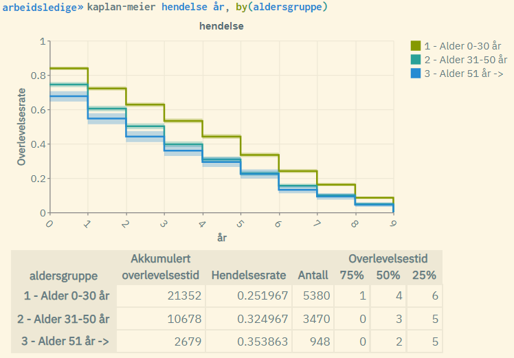
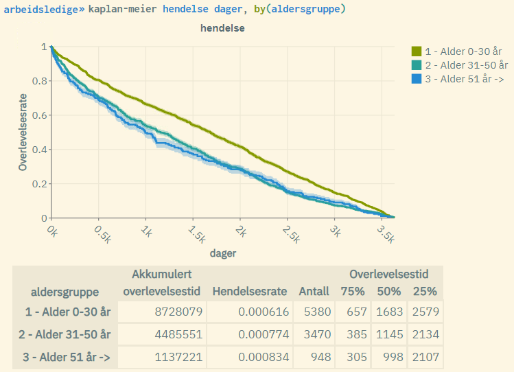
Explanation of the figure:

• The curves are given by the Kaplan-Meier formula for each age group. The youngest age group performs the best with a higher “survival rate” (are less likely to become unemployed over time).
• The shaded areas represent the standard log-log 5% confidence interval associated with the survival rate for each age group. These will be less visible in larger populations.
• “Akkumulert overlevelsestid”: Cumulative survival time, often referred to as “time at risk”. This is the sum of time measured over all units in the population (within each age group).
• “Hendelsesrate”: Event rate. This is the number of events occurred (number of units with event = 1) divided by cumulative survival time.
• “Antall”: Population size, i.e. the number of units (for each age group).
• “75%”: Time measured where survival rate = 0.75 (for each age group).
• “50%”: Time measured where survival rate = 0.5 (for each age group). Also known as “median survival time”.
• “25%”: Time measured where survival rate = 0.25 (for each age group).